TL;DR
The last post took a 0.8B SQL agent from 1/220 to 46/220 by copying a big teacher one token at a time. This one asks a simpler question: what if the student also got to see part of the teacher's uncertainty, not just its final pick? I kept everything else fixed: the harness, the 220-task eval, the action schema, the 0.8B student. I only changed the signal it learned from.
I scored the teacher's frozen traces, saved the top 20 token probabilities at each position plus a little leftover mass for everything else, and compared plain weighted hard-token training against top-k soft-label distillation. The best run hit 55/220, up from 46/220 for the hard-token student and 49/220 for the combined hard-token run.
The headline is not the interesting part. Soft labels actually hurt in two of the eight runs. And the best teacher was not the strongest one. A weaker same-family model, Qwen at 96/220, agreed with its own traces far better than the stronger model, GPT at 115/220, so its probabilities taught the student more cleanly. The win came from mixing both.
One honest caveat up front: I never had GPT's own token probabilities. The GPT traces here are scored by Qwen, so they are a proxy, not true GPT logit distillation.
What I Wanted To Test
I am trying to make small models better at narrow tasks. Same SQL repair agent as before. Hand it a user issue and some buggy SQL, and it can inspect a SQLite database, run SQL probes, read what comes back, and submit corrected SQL. The score comes from hidden deterministic tests, not an LLM judge.
The earlier hard-token run already showed the small model can run the loop, which was interesting on its own. The base model mostly repeated actions and never submitted. After hard-token SFT it inspected, queried, and submitted a lot more.
But hard-token training is blunt. If the teacher writes a token, the student is trained to copy that token. It does not see whether the teacher was confident, whether there were plausible alternatives, or whether the next-best token was almost as good. In SQL, that uncertainty can matter around table names, column names, predicates, joins, string values, and structured action syntax.
So the question for this post was:
Does top-k soft-label distillation improve the same 0.8B SQL agent when the traces and benchmark stay fixed?
I also wanted to test two starting points. One is the base unsloth/Qwen3.5-0.8B model. The other is the Qwen3.5-0.8B hard-token adapter trained on Qwen3.5-35B-A3B 8-bit successful trajectories. In other words: should soft-label training start from scratch, or should it continue from the hard-token student?
The SQL-Agent Problem
I kept the problem setup identical to the hard-token post. Each task has a user issue, a buggy SQL query, and a SQLite database. The model can choose structured actions: inspect schema, run SQL, or submit final SQL. A task succeeds only when the final submitted SQL passes the hidden tests.
Here is the same kind of small-but-real SQL repair task:
Database: chinook
User issue: I want to find the latest track_id and use that id to filter records in the track table.
Buggy SQL:
WITH vars AS (SELECT COUNT(*) AS vars_id FROM track)
SELECT * FROM track WHERE track_id = vars_id
The bug is not about formatting. COUNT(*) is not the latest id. The repair is closer to MAX(track_id), but the model has to discover that while operating a tool loop. It may need to inspect the schema, run a probe query, read the observation, and then submit final SQL in the exact structured format the harness accepts.
BAML, Boundary Markup Language, is still the structured-output layer around the prompt. It pins down the decision schema and builds the model request. I do not train the student on free-form teacher prose. It learns canonical JSON decisions: a short draft plus an executable output action.
{"draft":"Need schema first.","output":{"action":"inspect_schema"}}
{"draft":"Test a candidate query.","output":{"action":"run_sql_query","sql":"SELECT ..."}}
{"draft":"Submit corrected SQL.","output":{"action":"submit_sql","sql":["SELECT ..."]}}
Every eval used the same settings as the hard-token post, so the only thing that moved was the training signal:
| Eval setting | Value | | --- | --- | | Held-out eval split | 220 SQL repair tasks | | Max turns | 8 | | Local eval sequence cap | 8192 total tokens | | Max generated tokens per model call | 512, reserved inside the local sequence cap | | Temperature | 0.0 | | Task timeout | 180 seconds | | Scoring | deterministic hidden SQL tests |
Two of these deserve a note. The 8192 sequence cap is the whole prompt-plus-generation budget: system prompt, task, prior actions, schema, query results, the structured-output instructions, and the generation reserve all share it. I list max generated tokens separately because it caps the size of a single model call: the student can read a long state, but it still has to emit one compact action per turn.
The eval table uses these terminal outcomes and behavior metrics:
| Category or metric | Meaning |
| --- | --- |
| submitted but wrong | The model reached submit_sql, but the SQL failed hidden tests |
| SQL-error tasks | At least one model-issued SQL probe errored during the loop; this is not mutually exclusive with the final task outcome |
| parse failures | The output did not parse as a valid BAML action |
| repeat stops | The harness stopped the run because the model repeated actions |
| max-turn stops | The model used all 8 turns without solving the task |
| runtime errors | Process-level failures or timeouts |
I am spelling this out because the best students are not mainly failing on JSON. They reach submit_sql just fine. The real problem is SQL judgment and recovering when a probe goes sideways.
The Training Idea
With hard-token distillation, the student gets one target token at each position. Soft-label distillation hands it a small probability distribution instead.
For example, imagine the teacher target contains a table token like ... FROM users .... Hard-token training says: the next token is users.
Soft-label training can say:
| Token option | Teacher probability |
| --- | ---: |
| users | 0.72 |
| customers | 0.12 |
| accounts | 0.06 |
| orders | 0.03 |
| everything else | 0.07 |
That is a richer signal. The chosen token still matters, but the student also sees that some alternatives were closer than others.
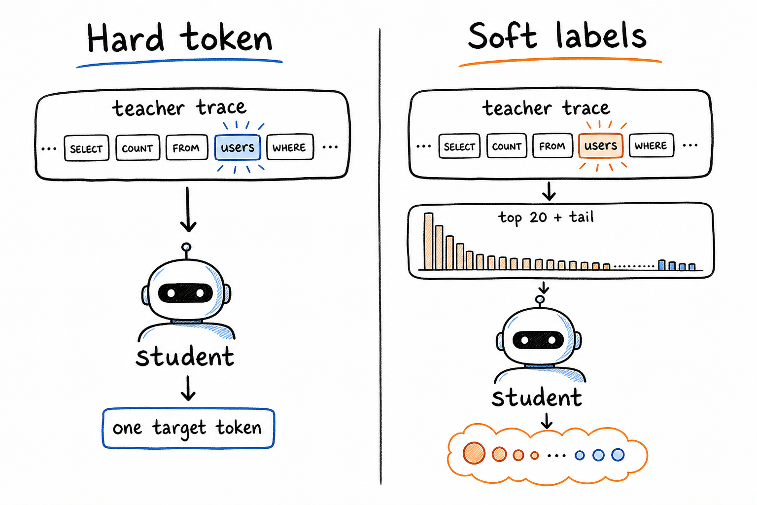
For a large language model, storing full-vocabulary probabilities is expensive. A vocabulary can have hundreds of thousands of tokens, and each teacher decision has many assistant target positions. So I used a practical sparse version: top 20 teacher token probabilities at each assistant target position, plus residual tail mass for all other tokens.
The tail matters. If the saved top 20 probabilities sum to 0.996, the missing 0.004 is still part of the teacher distribution. Renormalizing the top 20 to 1.0 would make the target artificially overconfident. I wanted the training target to remember that the unsaved vocabulary still had some probability mass.
This is still off-policy: the student learns from traces I collected earlier and never acts while I am scoring them.
A Small Educational Code Walkthrough
The easiest way to understand this post is to follow one row through the pipeline. The important point is that I did not create a new agent environment for soft labels. I reused the same successful teacher decisions from the hard-token trajectory run, rendered them with the same BAML prompt shape, then added probability information on the assistant target tokens.
The hard-token supervised fine-tuning (SFT) row looked like this. SFT means training the model on input-output examples, where the loss is only applied to the answer tokens I want the model to learn.
row = {
    "messages": conversation_before_teacher_decision + [
        {"role": "assistant", "content": canonical_decision_json(teacher_decision)}
    ],
    "teacher_draft": teacher_decision.draft,
    "teacher_action": teacher_decision.output,
}
For soft-label distillation, the row keeps the same canonical messages and teacher metadata, but adds teacher-forced token scores for assistant target positions. Teacher forcing means I feed the already-known target text to the probability model and ask, token by token, how likely that target was under the current context. The serialized data stores log probabilities, not raw probabilities, because they are numerically safer to write and train from.
row = {
    "messages": [..., {"role": "assistant", "content": target_decision_json}],
    "distillation": {
        "probability_model": "Qwen3.5-35B-A3B 8-bit",
        "top_k": 20,
        "row_weight": 1.18,
        "token_scores": [
            {
                "position": 1661,              # full-sequence token position
                "target_token_id": 412,
                "target_logprob": -0.21,
                "top_token_ids": [412, 879, 91],
                "top_logprobs": [-0.21, -2.81, -3.51],
                "top_mass": 0.90,
                "tail_mass": 0.10,
            }
        ],
    },
}
The scoring pass has one job: take a frozen row and stamp token probabilities onto it. I never ask the Qwen3.5-35B-A3B 8-bit scorer to write a new decision. I just render the prompt without the assistant answer, render the full sequence with it, and score the target part one token at a time.
prompt = chat_template(messages[:-1], add_generation_prompt=True)
full = chat_template(messages, add_generation_prompt=False)
prompt_ids = tokenize(prompt)
full_ids = tokenize(full)
target_ids = full_ids[len(prompt_ids):]
prefill_teacher_cache(prompt_ids[:-1])
driver_ids = [prompt_ids[-1]] + target_ids[:-1]
for i, target_id in enumerate(target_ids):
    logits = qwen_35b(driver_ids[i]).logits
    logprobs = log_softmax(logits)
    top_ids, top_logprobs = top_k(logprobs, k=20)
    save_token_score(
        position=len(prompt_ids) + i,
        target_token_id=target_id,
        target_logprob=logprobs[target_id],
        top_token_ids=top_ids,
        top_logprobs=top_logprobs,
        tail_mass=1.0 - sum(exp(top_logprobs)),
    )
The assistant-only masking stays the same as the hard-token run. Prompt tokens are context. Assistant target tokens are supervision. This matters more in an agent than in a plain question-answer task, because the prompt contains schema observations, prior tool outputs, and SQL execution results. The model should condition on those tokens, not learn to predict them.
labels = full_ids.copy()
labels[: len(prompt_ids)] = -100
hard_ce = cross_entropy(student_logits, labels)
The trainer stores more tensors than ordinary SFT. Each batch still has input_ids, attention_mask, and masked labels, but it also has per-position weights, top-k token ids, top-k log probabilities, a top-k mask, and tail probabilities. Padding fills inactive positions with neutral values so the loss can ignore them cleanly.
batch = {
    "input_ids": pad(input_ids, pad_id),
    "attention_mask": pad(attention_mask, 0),
    "labels": pad(labels, -100),
    "position_weights": pad(position_weights, 0.0),
    "topk_token_ids": pad(topk_token_ids, [0] * top_k),
    "topk_logprobs": pad(topk_logprobs, [0.0] * top_k),
    "topk_mask": pad(topk_mask, [False] * top_k),
    "tail_probs": pad(tail_probs, 0.0),
}
Weighted hard-token fine-tuning is the control condition. It still trains on one chosen target token, but multiplies assistant-token cross-entropy by a confidence weight derived from the scorer's target log probability. A row the scorer finds easy can count more; a row it finds less likely can count less.
z = (mean_target_logprob - dataset_mean_logprob) / dataset_logprob_std
row_weight = clip(2 / (1 + exp(-z)), 0.25, 1.75)
loss = row_weight * hard_ce
The clip range [0.25, 1.75] keeps one messy row from hijacking a batch, while still letting confident rows count a good deal more than shaky ones.
Top-k soft-label distillation adds a probability-matching term. This is not exact production code, but it shows the shape of the loss:
teacher_top_probs = exp(top_logprobs) * topk_mask
teacher_top_probs *= (1.0 - tail_mass) / sum(teacher_top_probs)
student_logprobs = log_softmax(student_logits_at_target_positions)
student_top_logprobs = gather(student_logprobs, topk_token_ids)
student_tail_prob = 1.0 - sum(exp(student_top_logprobs))
topk_kl = sum(teacher_top_probs * (log(teacher_top_probs) - student_top_logprobs))
tail_kl = tail_mass * (log(tail_mass) - log(student_tail_prob))
loss = hard_ce + topk_kl + tail_kl
The direction is teacher to student: the teacher distribution is the target, and the student is penalized when it puts too little probability on that mass. In the real trainer, both cross-entropy and distillation are computed on shifted assistant target positions only.
The actual student training is still LoRA fine-tuning. LoRA means low-rank adaptation: the base model stays mostly frozen, and small trainable adapter matrices are attached to selected attention and MLP modules. That gave me a cheap way to compare many runs without fully fine-tuning the 0.8B model every time.
student = load_student("unsloth/Qwen3.5-0.8B", max_seq_length=4096)
student = add_lora_adapters(
    student,
    rank=32,
    alpha=32,
    target_modules=[
        "q_proj", "k_proj", "v_proj", "o_proj",
        "gate_proj", "up_proj", "down_proj",
    ],
)
trainer_class = make_trainer_class(Trainer, soft_label_args)
trainer = trainer_class(
    model=student,
    train_dataset=scored_train_examples,
    eval_dataset=scored_validation_examples,
    data_collator=distillation_collator,
    batch_size=1,
    gradient_accumulation_steps=8,
    learning_rate=5e-5,
    epochs=3,
)
trainer.train()
adapter = save_lora_adapter(student)
This mirrors the local implementation: make_trainer_class returns a Hugging Face Trainer subclass with the saved sparse top-k plus residual-tail loss. That is different from TRL's online DistillationTrainer path, where the teacher can score inside the trainer. For the soft-label runs, the hard cross-entropy weight was 1.0, the distillation loss weight was 1.0, and temperature was 1.0. I kept temperature simple on purpose because the sparse artifacts were produced at temperature 1.0 and I did not want this post to become a temperature-scaling experiment.
The final evaluation is a real rollout, not teacher forcing. The trained adapter goes back into the same SQL-agent harness and has to solve the 220 held-out tasks by acting turn by turn.
for task in held_out_eval_tasks:
    state = start_sql_agent_task(task)
    for turn in range(8):
        messages = render_baml_messages(state)
        decision = model_with_adapter.generate_action(
            messages,
            max_new_tokens=512,
            temperature=0.0,
        )
        state = execute_action_and_append_observation(state, decision)
        if state.solved or state.stopped:
            break
    results.append(score_final_submission(state))
That last step is where a lot of offline distillation ideas quietly break. Teacher forcing measures whether the student can predict the teacher's next action in a teacher-style context. Rollout eval measures whether the student can survive its own previous actions, pick useful SQL probes, avoid repeating itself, and submit correct SQL. This post is about the second number.
How The Experiment Runs
This part is easy to misread as on-policy distillation, so I will say it plainly up front: it is not. The student never generates the tokens being scored. It only learns, after the fact, from traces the teacher already left behind. With that out of the way, here is the shape of the whole thing.
The data is a scoring pass over those frozen successful traces. The teacher's actions already exist; the probability model just asks, "how likely did each of those chosen tokens look, given the context?" It never writes a new decision. I kept the two scored datasets separate (GPT traces scored by Qwen, and Qwen traces scored by Qwen) and filtered on the full rendered sequence length, because schema observations and earlier tool outputs are part of what the student has to absorb, not just the final answer. Boundary: the GPT traces are Qwen-proxy-scored, not GPT's own probabilities, and the student never acts while I am scoring.
Then there are three ways to train on that scored data:
- Weighted hard-token fine-tuning (the control). Still one chosen token per position, but each row is weighted by how confident the scorer was. This is just SFT with a confidence knob. Boundary: this is not soft-label distillation. The student sees the weight, never the top-k distribution.
- Top-k soft-label distillation (the method this post is about). Same hard target, plus a second signal asking the student to spread probability over the same top-k alternatives the scorer saw, while reserving the leftover mass for everything else. Boundary: off-policy and teacher-forced over frozen traces. It is not on-policy, and the teacher never scores the student's own samples.
- Combined teacher-source mix. Concatenate the GPT-proxy rows and the Qwen-self rows, shuffle, and train the base student two ways. Boundary: this is data mixing across teachers, not one merged probability distribution. Each row keeps its own scorer.
That mix is what eventually gives the cleanest win. It's also the least mysterious result in the post: more diverse successful traces, plus a richer per-token target, gave the small base model more to work with than either source alone.
Dataset And Filtering
I did not regenerate teacher traces for this post, and that was on purpose. The traces were frozen from the hard-token run, so the comparison stays focused on the supervision signal and not on a fresh data-generation run.
In that earlier data-generation pass, both teachers ran on the same 879 train tasks. GPT 5.5 medium solved 446/879 and produced 1046 SFT rows. Qwen3.5-35B-A3B 8-bit solved 394/879 and produced 1232 rows because its successful traces were longer. On the 220-task eval, GPT 5.5 medium was stronger at 115/220 versus 96/220 for Qwen3.5-35B-A3B 8-bit, so the Qwen path here is a same-family test, not the strongest-teacher path.
There are two trace sources:
| Trace source | Probability source | What it means | | --- | --- | --- | | GPT 5.5 medium successful traces | Qwen3.5-35B-A3B 8-bit | Proxy scoring. These are not GPT 5.5 medium's internal probabilities. They are Qwen3.5-35B-A3B 8-bit probabilities while teacher-forcing GPT's chosen actions. | | Qwen3.5-35B-A3B 8-bit successful traces | Qwen3.5-35B-A3B 8-bit | Same-family self-scoring. The same model family produced and scored the traces. |
The proxy caveat is important. True GPT 5.5 medium soft labels would require GPT 5.5 medium token probabilities. I did not have that. So the GPT trace experiment asks a narrower question: can a same-family Qwen scorer add useful signal to GPT's chosen actions?
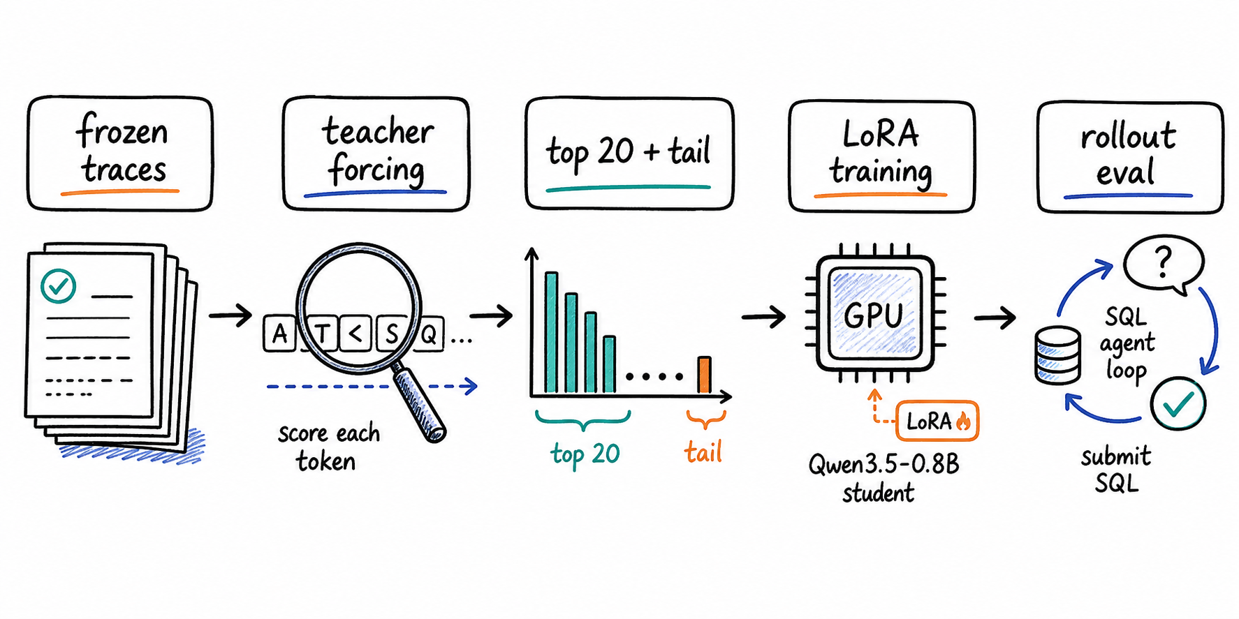
For each row, I rendered the BAML prompt the harness actually uses. Then I teacher-forced the known assistant target through Qwen3.5-35B-A3B 8-bit and stored token scores only for the assistant target positions.
Before training anything, I had two questions about the scored data itself. How much of it fit the 4096-token budget? And how well did the Qwen scorer actually agree with each trace source?
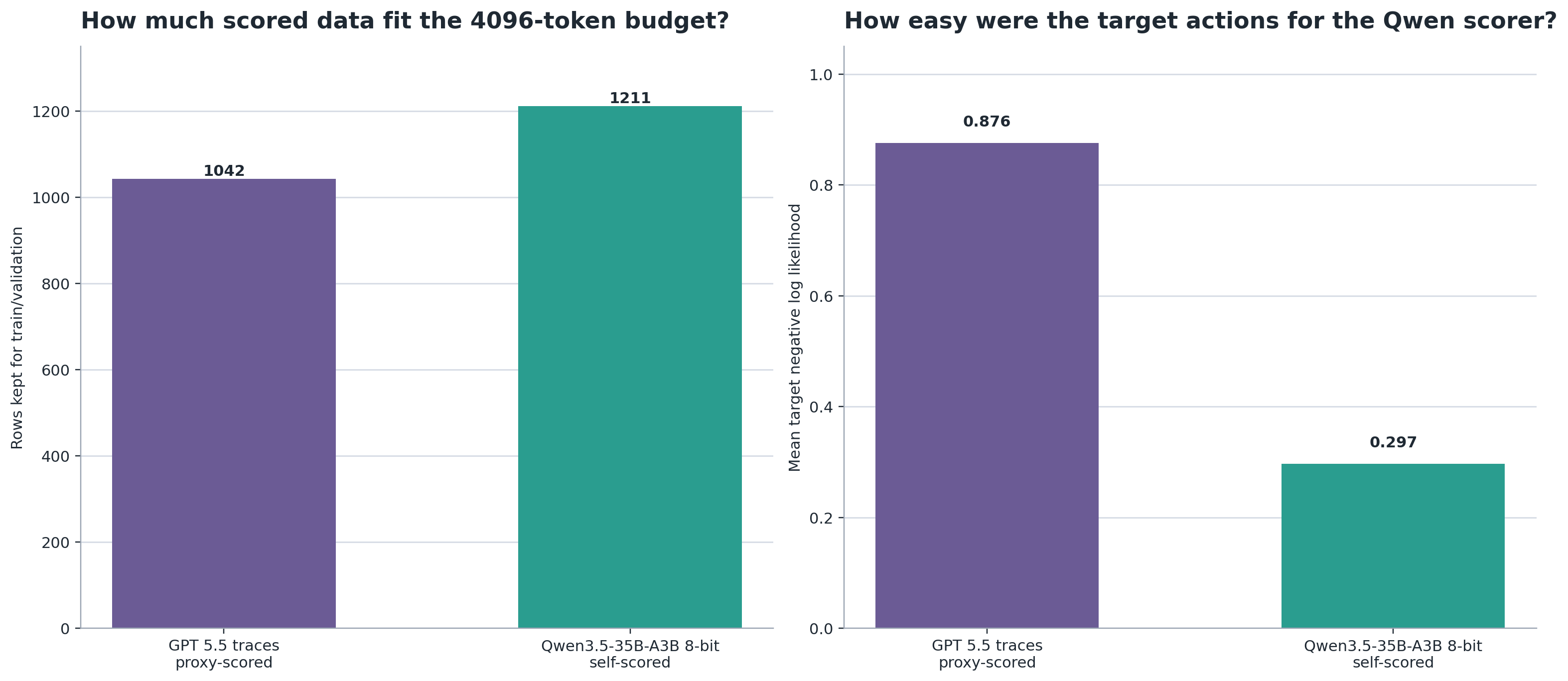
In the right-hand panel, lower negative log likelihood is better. It means the probability model found the target actions easier to explain. That is why the Qwen self-scored data looks so different from the GPT proxy-scored data: Qwen3.5-35B-A3B 8-bit was much more confident about its own traces than about GPT 5.5 medium's traces.
| Scored dataset | Source rows | Kept at 4096 | Train/validation | Mean prompt tokens | Mean target tokens | P95 full sequence | Mean target negative log likelihood | Target in top 20 | | --- | ---: | ---: | ---: | ---: | ---: | ---: | ---: | ---: | | GPT 5.5 medium traces, proxy-scored by Qwen3.5-35B-A3B 8-bit | 1046 | 1042 | 990 / 52 | 1658 | 87 | 3171 | 0.876 | 98.56% | | Qwen3.5-35B-A3B 8-bit traces, self-scored | 1232 | 1211 | 1151 / 60 | 1879 | 79 | 3403 | 0.297 | 100.00% |
Qwen3.5-35B-A3B 8-bit found its own traces much easier to explain than the GPT traces. The mean target negative log likelihood was 0.297 for Qwen self-scored rows versus 0.876 for GPT proxy-scored rows. The target token appeared inside the stored top 20 for 100.00% of Qwen self-scored target positions and 98.56% of GPT proxy-scored positions.
The combined dataset had 2278 source rows, 2253 rows after the 4096-token filter, 2141 train rows, and 112 validation rows. I shuffled the combined rows with a fixed seed before splitting so the validation set would not depend on source order.
Training Setup
The main grid was 2 x 2 x 2: two trace sources, two training methods, and two student starts.
| Axis | Values |
| --- | --- |
| Student model | unsloth/Qwen3.5-0.8B |
| Student start | base model; Qwen3.5-0.8B hard-token trajectory adapter trained on Qwen3.5-35B-A3B 8-bit rows |
| Trace source | GPT 5.5 medium successful traces; Qwen3.5-35B-A3B 8-bit successful traces |
| Probability model | Qwen3.5-35B-A3B 8-bit |
| Training methods | weighted hard-token fine-tuning; top-k soft-label distillation |
After those eight runs, I added two combined-teacher runs from the base model: one weighted hard-token run and one soft-label run. That gives ten trained students in total. I did not add combined warm-start runs in this post because the first eight runs already showed that warm-start behavior depended strongly on the trace source, and I wanted the combined-data test to answer a simpler question: if I start from the base model, does mixing teacher sources help?
The training recipe stayed close to the hard-token trajectory baseline: LoRA rank 32, LoRA alpha 32, target modules q_proj, k_proj, v_proj, o_proj, gate_proj, up_proj, and down_proj, learning rate 5e-5, batch size 1, gradient accumulation 8, three epochs, bf16 on an NVIDIA GPU, Unsloth, and FlashAttention 2 where available. I used a 5% validation split, no packing, seed 42, and a 4096-token full training sequence cap.
The soft-label loss used temperature 1.0, hard cross-entropy weight 1.0, and distillation loss weight 1.0. The implementation keeps the stored top-k mass and the residual tail mass. That is just a numerical correction for sparse serialized probabilities.
The training size was not exactly the same for every run. GPT proxy-scored runs had 990 train rows, Qwen self-scored runs had 1151 train rows, and combined runs had 2141 train rows. With batch size 1 and gradient accumulation 8, that became 372, 432, and 804 optimizer updates over three epochs.
In the table below, Base means the unfine-tuned unsloth/Qwen3.5-0.8B model. GPT proxy means GPT 5.5 medium traces scored by Qwen3.5-35B-A3B 8-bit. Qwen self means Qwen3.5-35B-A3B 8-bit traces scored by the same Qwen3.5-35B-A3B 8-bit model. Combined means those two scored row sets were concatenated before training.
| Student start | Data | Method | Train rows | Optimizer updates | Final validation loss | Train time | | --- | --- | --- | ---: | ---: | ---: | ---: | | Base | GPT proxy | weighted hard | 990 | 372 | not captured in synced training log | not captured | | Base | GPT proxy | soft label | 990 | 372 | 0.6795 | 24.5 min | | Base | Qwen self | weighted hard | 1151 | 432 | 0.2544 | 27.6 min | | Base | Qwen self | soft label | 1151 | 432 | 0.4902 | 29.4 min | | Hard-token trajectory warm start | GPT proxy | weighted hard | 990 | 372 | 0.3547 | 23.0 min | | Hard-token trajectory warm start | GPT proxy | soft label | 990 | 372 | 0.6592 | 24.2 min | | Hard-token trajectory warm start | Qwen self | weighted hard | 1151 | 432 | 0.2956 | 27.5 min | | Hard-token trajectory warm start | Qwen self | soft label | 1151 | 432 | 0.4950 | 29.6 min | | Base | Combined | weighted hard | 2141 | 804 | 0.3478 | 51.8 min | | Base | Combined | soft label | 2141 | 804 | 0.5684 | 55.2 min |
A small warning on this table: validation losses are useful inside one objective, but they are not directly comparable between weighted-hard and soft-label runs because the losses include different terms. The base Qwen self-scored weighted-hard run had the lowest validation loss in the table, but it solved only 40/220. The best rollout score came from the combined soft-label run, even though its validation loss was higher.
A high-memory preparation machine was useful for loading and scoring Qwen3.5-35B-A3B 8-bit locally, but exact teacher-forced scoring was slow: about 60 minutes for the GPT trace set and 41 minutes for the Qwen trace set. Student training belonged on the NVIDIA GPU. The single-source GPU trainings with recorded runtimes were roughly 23 to 30 minutes each, and the larger combined runs took about 52 minutes for weighted hard tokens and 55 minutes for soft labels.
Results As Research Questions
The first result chart I made tried to put everything in one place. That was confusing because it mixed two different questions: what happens when I start from the base model, and what happens when I continue from the hard-token trajectory model?
So I split the results by the actual research questions.
For scale, the teacher/baseline picture from the fixed 220-task eval was this:
| Model | Role in this post | Success | Submitted | Avg turns | | --- | --- | ---: | ---: | ---: | | GPT 5.5 medium | Strong trace teacher from the hard-token data-generation pass | 115/220 | 220 | 2.53 | | GPT 5.4 mini | Hosted baseline on the same fixed eval | 105/220 | 220 | 2.14 | | Qwen3.5-35B-A3B 8-bit | Same-family trace teacher and probability model | 96/220 | 202 | 3.57 | | Qwen3.5-0.8B hard-token trajectory student | Warm-start checkpoint | 46/220 | 155 | 3.48 | | Base Qwen3.5-0.8B | No fine-tuning | 1/220 | 1 | 2.39 |
The point of this top-k soft-label experiment was not to beat the teachers. The point was to ask whether a richer supervision signal can move the 0.8B student further under the same harness.
First: if I start from the base unsloth/Qwen3.5-0.8B model, what helps?
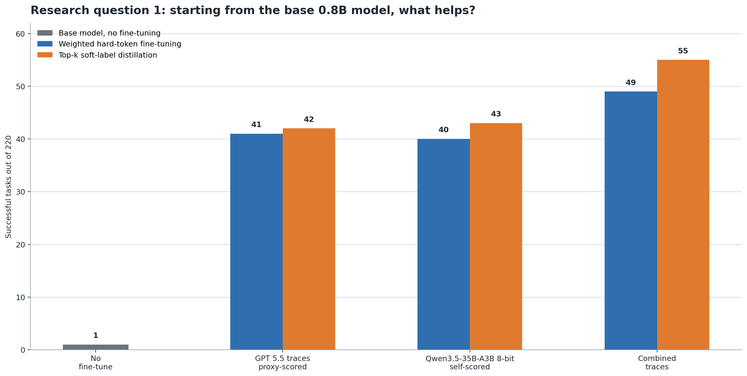
Every training run beat the no-fine-tune baseline of 1/220. Single-source GPT 5.5 medium traces and single-source Qwen3.5-35B-A3B 8-bit traces were close, 41 to 43 solved tasks depending on method. The bigger jump came from combining teacher sources. Combined weighted hard-token fine-tuning reached 49/220, and combined top-k soft-label distillation reached 55/220. That is about a 25% solve rate, modest in absolute terms and well under the strongest teacher's 115/220. But this series is about how far a 0.8B model can climb from a near-zero base, not about catching the teacher.
For the base model, the clearest answer is: use both teacher sources, and soft labels beat weighted hard tokens on that combined data.
Second: if I already have the hard-token trajectory student, should I continue training it?
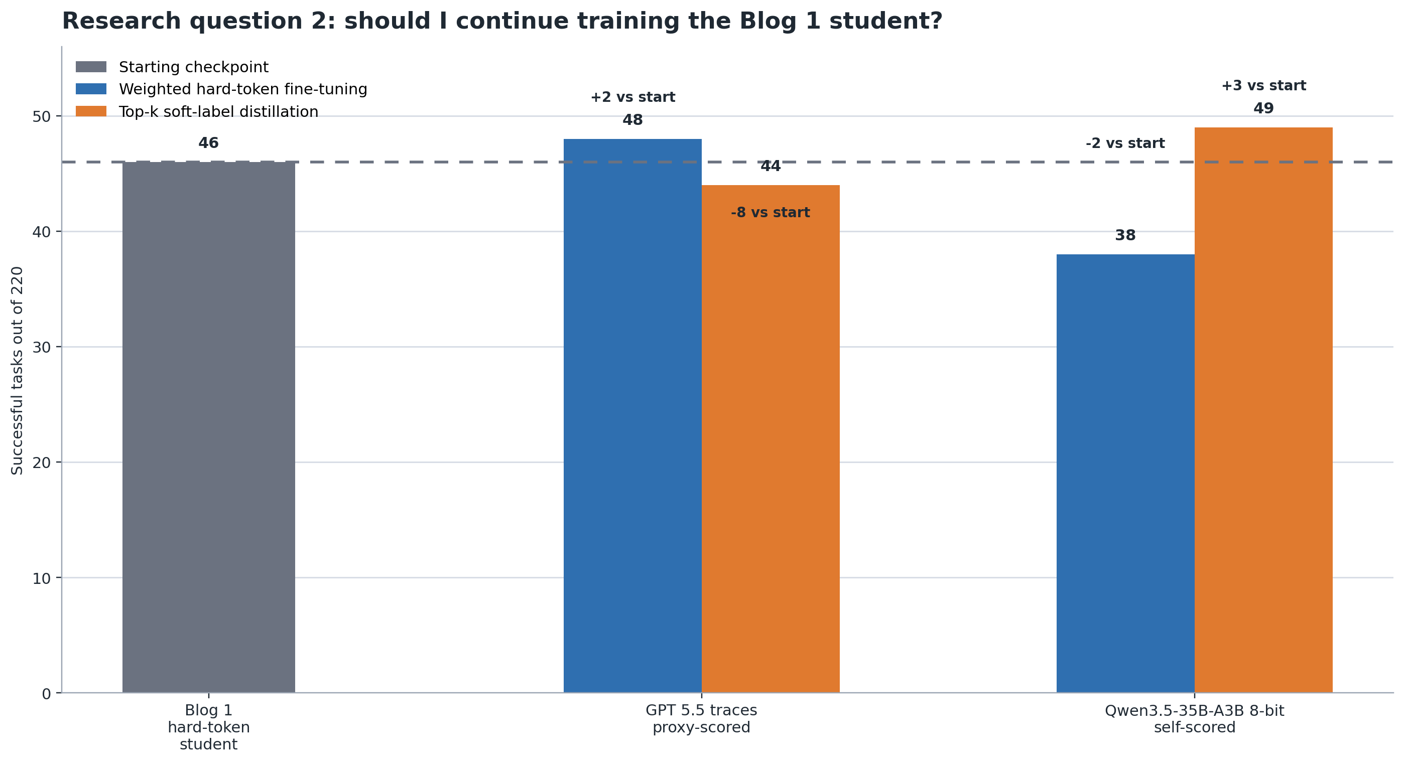
Here the answer is more subtle. The starting checkpoint was already 46/220. Continuing on GPT 5.5 medium traces with weighted hard-token fine-tuning gave a small gain to 48/220, while soft-label distillation on the same GPT traces dropped to 44/220. On Qwen3.5-35B-A3B 8-bit self-scored traces, the direction flipped: weighted hard-token fine-tuning dropped to 38/220, while soft-label distillation improved to 49/220.
The part I did not expect: soft labels only paid off where the scorer agreed with the trace. Qwen3.5-35B-A3B 8-bit scored just 96/220 as a teacher, weaker than GPT at 115/220. But its probabilities lined up with its own traces, so soft labels worked there at 49/220 and actually hurt on the proxy-scored GPT traces at 44/220. Alignment beat raw teacher strength.
Third: what changed in the agent loop?
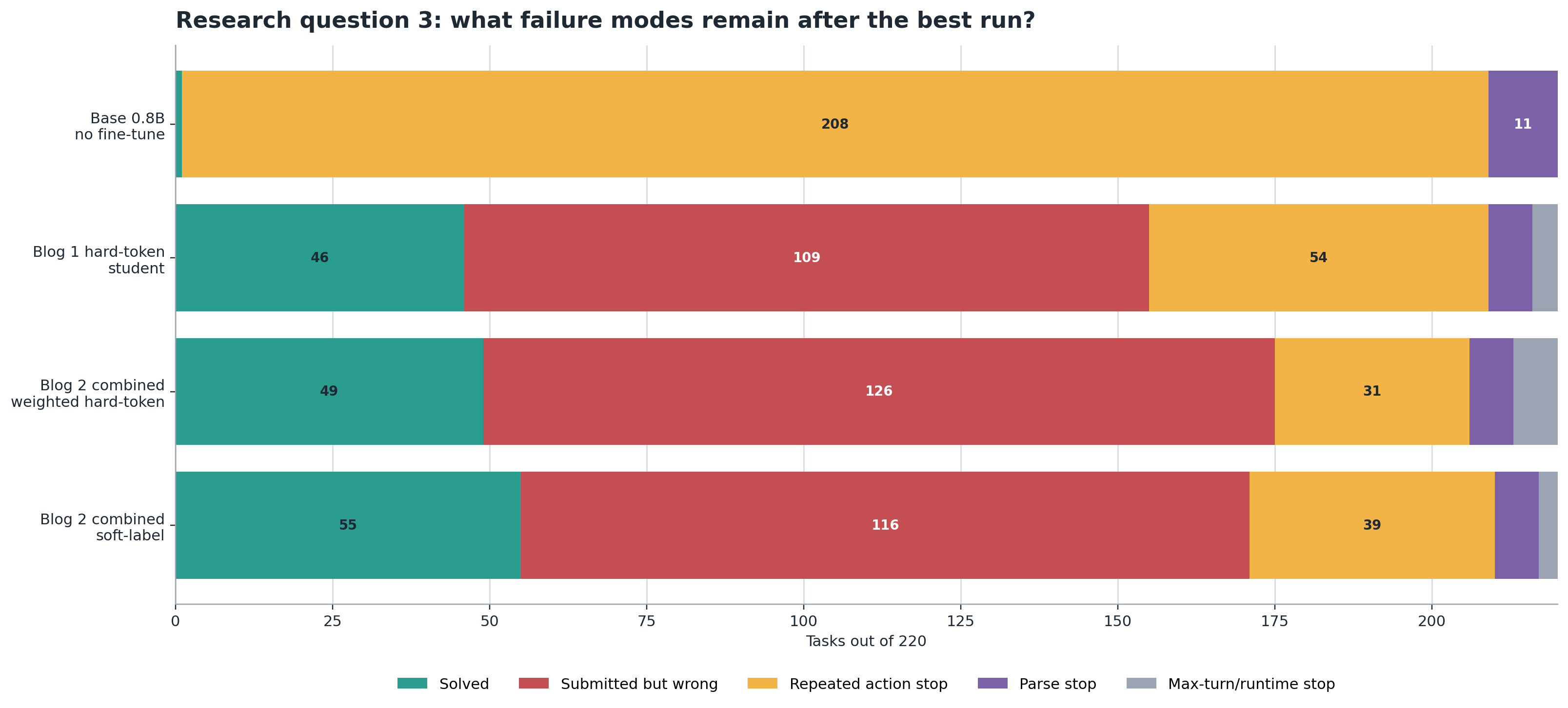
The base model almost never submitted at all. Hard-token trajectory SFT taught it to actually enter the loop and submit, but a lot of those submissions were wrong. The combined soft-label run pushed success up again, and it is the best run in the post. Even so, it submitted 171 tasks and solved 55, so 116 submitted queries failed the hidden tests. It still had 39 repeated-action stops too.
That is the honest shape of the result. The model is not mainly failing because it cannot emit valid BAML actions. It is failing because it still makes bad SQL decisions and sometimes gets stuck in the loop.
Turn count was the cleanest behavior signal I had. The combined soft-label run averaged 3.39 turns, almost the same as the hard-token warm start at 3.48, so the gain did not come from taking more steps. It came from a slightly better mix of actions: more solved submissions than the hard-token warm start, fewer wrong submissions than the combined weighted-hard run, fewer SQL errors, and fewer max-turn stops. I did not log exact generated-token counts per eval call, so I am not reporting output-token numbers here. The token stats I can report cleanly are on the training side: prompt tokens, target tokens, full-sequence length, and top-k coverage.
Exact Numbers Behind The Charts
The chart is the reading path. These tables are the audit path for the baselines and trained students shown in the charts. Submitted includes successful submissions and wrong submissions. Wrong submits is submitted - success.
| Student start | Data source | Method | Success | Submitted | Wrong submits | Avg turns | | --- | --- | --- | ---: | ---: | ---: | ---: | | Base Qwen3.5-0.8B | No fine-tuning | baseline | 1/220 | 1 | 0 | 2.39 | | Hard-token trajectory warm start | Qwen3.5-35B-A3B 8-bit hard-token rows | starting checkpoint | 46/220 | 155 | 109 | 3.48 | | Base Qwen3.5-0.8B | GPT 5.5 traces proxy-scored by Qwen3.5-35B-A3B 8-bit | weighted hard-token fine-tuning | 41/220 | 198 | 157 | 2.60 | | Base Qwen3.5-0.8B | GPT 5.5 traces proxy-scored by Qwen3.5-35B-A3B 8-bit | top-k soft-label distillation | 42/220 | 185 | 143 | 2.76 | | Base Qwen3.5-0.8B | Qwen3.5-35B-A3B 8-bit traces self-scored | weighted hard-token fine-tuning | 40/220 | 155 | 115 | 3.46 | | Base Qwen3.5-0.8B | Qwen3.5-35B-A3B 8-bit traces self-scored | top-k soft-label distillation | 43/220 | 158 | 115 | 3.29 | | Hard-token trajectory warm start | GPT 5.5 traces proxy-scored by Qwen3.5-35B-A3B 8-bit | weighted hard-token fine-tuning | 48/220 | 202 | 154 | 2.68 | | Hard-token trajectory warm start | GPT 5.5 traces proxy-scored by Qwen3.5-35B-A3B 8-bit | top-k soft-label distillation | 44/220 | 192 | 148 | 3.05 | | Hard-token trajectory warm start | Qwen3.5-35B-A3B 8-bit traces self-scored | weighted hard-token fine-tuning | 38/220 | 148 | 110 | 3.78 | | Hard-token trajectory warm start | Qwen3.5-35B-A3B 8-bit traces self-scored | top-k soft-label distillation | 49/220 | 151 | 102 | 3.46 | | Base Qwen3.5-0.8B | Combined GPT proxy + Qwen self-scored rows | weighted hard-token fine-tuning | 49/220 | 175 | 126 | 3.36 | | Base Qwen3.5-0.8B | Combined GPT proxy + Qwen self-scored rows | top-k soft-label distillation | 55/220 | 171 | 116 | 3.39 |
SQL-error tasks is non-exclusive: it means at least one SQL probe errored during the loop, and it can overlap with the final task outcome.
| Student start | Data source | Method | SQL-error tasks | Parse failures | Repeat stops | Max-turn stops | Runtime errors | | --- | --- | --- | ---: | ---: | ---: | ---: | ---: | | Base Qwen3.5-0.8B | No fine-tuning | baseline | 0 | 11 | 208 | 0 | 0 | | Hard-token trajectory warm start | Qwen3.5-35B-A3B 8-bit hard-token rows | starting checkpoint | 5 | 7 | 54 | 4 | 0 | | Base Qwen3.5-0.8B | GPT 5.5 traces proxy-scored by Qwen3.5-35B-A3B 8-bit | weighted hard-token fine-tuning | 39 | 8 | 13 | 1 | 0 | | Base Qwen3.5-0.8B | GPT 5.5 traces proxy-scored by Qwen3.5-35B-A3B 8-bit | top-k soft-label distillation | 23 | 4 | 30 | 1 | 0 | | Base Qwen3.5-0.8B | Qwen3.5-35B-A3B 8-bit traces self-scored | weighted hard-token fine-tuning | 10 | 9 | 54 | 2 | 0 | | Base Qwen3.5-0.8B | Qwen3.5-35B-A3B 8-bit traces self-scored | top-k soft-label distillation | 10 | 4 | 54 | 4 | 0 | | Hard-token trajectory warm start | GPT 5.5 traces proxy-scored by Qwen3.5-35B-A3B 8-bit | weighted hard-token fine-tuning | 35 | 5 | 13 | 0 | 0 | | Hard-token trajectory warm start | GPT 5.5 traces proxy-scored by Qwen3.5-35B-A3B 8-bit | top-k soft-label distillation | 23 | 3 | 24 | 1 | 0 | | Hard-token trajectory warm start | Qwen3.5-35B-A3B 8-bit traces self-scored | weighted hard-token fine-tuning | 14 | 7 | 61 | 4 | 0 | | Hard-token trajectory warm start | Qwen3.5-35B-A3B 8-bit traces self-scored | top-k soft-label distillation | 13 | 8 | 54 | 7 | 0 | | Base Qwen3.5-0.8B | Combined GPT proxy + Qwen self-scored rows | weighted hard-token fine-tuning | 14 | 7 | 31 | 6 | 1 | | Base Qwen3.5-0.8B | Combined GPT proxy + Qwen self-scored rows | top-k soft-label distillation | 12 | 7 | 39 | 3 | 0 |
Failure Analysis
If I only looked at the combined base-model run, the story would be too clean: mixed teacher data plus soft labels wins, full stop. The split charts show the real, messier shape. The headline lesson is the counterintuitive one. A weaker teacher taught the student better than the stronger one, because its probabilities agreed with its own traces. Soft labels helped most on same-family Qwen paths and clearly when both teacher sources were combined. They helped less on GPT traces that were only proxy-scored by Qwen, and they actually hurt the GPT warm-start cell.
This makes sense to me. Qwen3.5-35B-A3B 8-bit probabilities explain Qwen3.5-35B-A3B 8-bit actions well, which gives the Qwen3.5-0.8B student a cleaner signal to imitate.
Rollout still dominates. Teacher forcing asks whether the student can predict the teacher's next action given a teacher-style context. The eval harness asks whether the student can recover after its own previous actions, choose useful probes, avoid loops, and submit correct SQL. Those are related, but they are not the same.
Validation loss shows the same gap from another angle. The combined soft-label run reached 55/220 with a higher validation loss, 0.5684, than the combined hard-token run's 0.3478 at 49/220. And the base Qwen self-scored hard-token run had the lowest loss in the table, 0.2544, yet solved only 40/220. Lower teacher-forced loss was just not the same as a better agent.
The combined-teacher result is the most useful result in the post. GPT 5.5 medium traces pushed the student toward submitting more often. Qwen3.5-35B-A3B 8-bit traces gave same-family, easier-to-score trajectories, but also more loopiness. The mixed soft-label run did not magically inherit only the best behavior from both. It still had repeat stops. But it reached the best success score, with fewer SQL execution errors and fewer max-turn stops than the mixed hard-token run.
The weighted-hard control also taught me something. Weighting a row by scorer confidence is cheaper than training against sparse probability distributions, and on GPT proxy-scored warm-start data it was the best cell. But it cannot teach the student about nearby alternatives at each token position. It only says, "copy this chosen token more or less strongly." Top-k soft labels are a better fit when the scorer is aligned with the trace source and when the data mix is broad enough to avoid over-specializing to one teacher style.
Hardware And Infrastructure Lessons
This post needed two different kinds of machine. Scoring meant holding Qwen3.5-35B-A3B 8-bit in memory and running it over frozen targets, so I used a high-RAM Mac where 128 GB of unified memory can keep the quantized teacher resident. It was not fast, but it let me do all the prep work locally before paying for GPU time.
Training wanted the opposite. LoRA fine-tuning is matrix heavy, forward and backward passes, attention kernels, optimizer steps, and the NVIDIA GPU was much faster even with less total memory, because those tensors stayed in VRAM and ran on CUDA kernels.
| Work | Hardware shape that helped | Observed time | | --- | --- | ---: | | Score GPT 5.5 medium traces with Qwen3.5-35B-A3B 8-bit | High-RAM preparation machine | about 60 min | | Score Qwen3.5-35B-A3B 8-bit traces with itself | High-RAM preparation machine | about 41 min | | Single-source student LoRA training | NVIDIA GPU | about 23-30 min | | Combined weighted-hard student LoRA training | NVIDIA GPU | about 52 min | | Combined soft-label student LoRA training | NVIDIA GPU | about 55 min |
The lesson I keep relearning: capacity and throughput are different problems. Big system RAM lets you fit things and prepare them. GPU VRAM plus CUDA lets you train them quickly. My workflow settled into doing everything I could on the Mac, and only firing up the remote GPU once the data and scripts were ready.
What I Learned
Soft-label distillation is worth testing for agent fine-tuning, but it needs rollout evaluation. Token-level uncertainty is a richer signal than hard tokens, but it is still local supervision. It does not automatically teach recovery after a wrong tool call, loop avoidance, or better SQL probing under new observations.
Proxy soft labels should be labeled honestly. The GPT rows here are not GPT's own probabilities. They are Qwen-scored (see the Dataset section). That is still a useful experiment, just not true GPT logit distillation.
A same-family teacher can be the better teacher even when it is not the strongest one. Alignment with the trace mattered more than the eval score.
Sparse top-k plus tail is a practical compromise. Full-vocabulary logits would be more complete, but they are expensive to store, move, and train against. Top 20 plus residual tail kept enough signal to make the target token visible almost everywhere.
Mixing teachers helped more than choosing one winner. The best result came from combining GPT 5.5 medium proxy-scored rows with Qwen3.5-35B-A3B 8-bit self-scored rows and training the base model with soft labels.
Conclusion
The answer is yes, but with conditions. Top-k soft-label distillation improved the 0.8B SQL agent in the best setup: combined GPT 5.5 medium proxy-scored rows plus Qwen3.5-35B-A3B 8-bit self-scored rows, trained into the base unsloth/Qwen3.5-0.8B student, reached 55/220. That beats the off-policy hard-token trajectory student at 46/220 and the combined hard-token run at 49/220.
But this is not a simple "soft labels always win" recipe. Teacher source, student initialization, probability alignment, and rollout behavior all mattered, and the teacher that won was not the one with the best eval score. The remaining failures are still agentic: wrong SQL, repeated actions, and imperfect recovery inside the loop.
That is why I like this benchmark for the series. The student can look good under teacher forcing and still fail when it has to act. The next useful experiment should keep the same harness and ask whether a new training idea improves the actual loop, not only the offline loss.